Deutsch
 Italiano
 Español
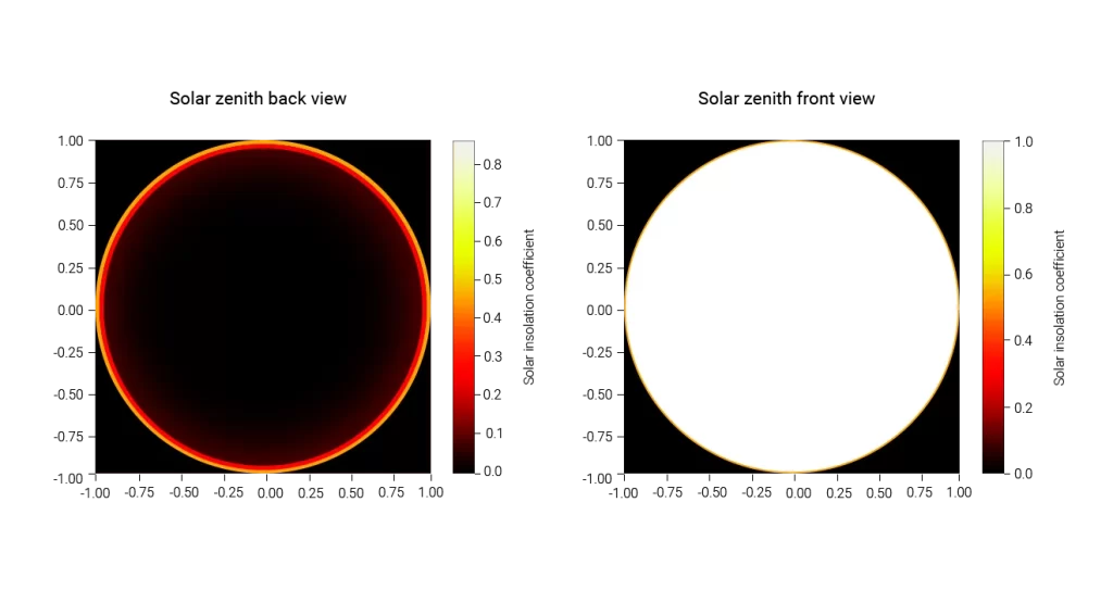
We can observe that in the daytime hemisphere, the solar irradiance factor is close to 1 in most regions, while in the nighttime hemisphere, there are regions where the solar irradiance factor is around 20° or more. To calculate the specific global average solar irradiance factor, the Earth’s surface can be divided into the following three parts:
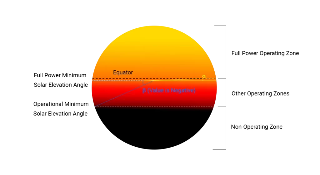
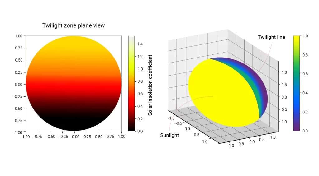
As shown in the diagram, the bright yellow region above the dividing line represents the full-power operating zone of solar panels, while the area between the bright yellow and red lines indicates the zone where solar panels operate at less than full power but are still functional. The black region represents the non-operational zone. The efficiency of solar panels on a global scale is essentially the integral of the solar irradiance factor over the Earth’s surface divided by the surface area of the sphere. In the full-power operating zone, the solar irradiance factor is 1, while in the non-operational zone, it is 0. Therefore, the formula can be expressed as:
Uniform Direct Irradiance Coefficient Formula:
Uniform Direct Irradiance Coefficient=(Spherical Surface AreaFull Power Working Area+Workable area direct irradiance coefficient)/Spherical Surface Area
That is, there is the following formula:
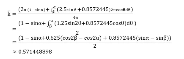
Where ˉ denotes the average direct irradiance coefficient, α and β are indicated in Figure 1.3. If we consider the Earth at this moment as a planet with a horizontal axial rotation where the North Pole is pointing towards the Sun, then α and β represent the latitudes where the two dividing lines are located (with negative values for latitudes in the southern hemisphere). Substituting α and β.

The calculated average direct irradiance coefficient is approximately 0.571449. This implies that for a planet entirely covered with solar panels, the total electricity generated by the solar panels would be approximately 0.571449× the number of solar panels × the solar energy utilization rate × 360 kW. For a planet with a 100% solar energy utilization rate, the expected annual electricity generation of a randomly positioned solar panel would be approximately 205.72 kW.
However, it’s essential to note that this value is theoretical. In practical scenarios, solar panels are deployed discretely rather than uniformly covering the entire spherical surface of a planet. Additionally, factors such as panel spacing and the presence of obstacles may further affect the actual efficiency. For instance, considering a solar panel every 3 degrees of latitude with 500 latitude lines from the South Pole to the North Pole, it’s practically challenging to achieve perfect coverage. Moreover, in polar regions, the presence of adjacent buildings with large orientation angles may limit the dense deployment of solar panels. Therefore, there might be discrepancies between theoretical and actual values. In a real-world measurement, the average direct irradiance coefficient of solar panels was found to be approximately 0.57109, representing a relative error of about 0.06% compared to the theoretical value. It is expected that various blueprints aiming for as uniform coverage as possible will have a relative error of no more than 0.1%.
Annual Average Electricity Generation Efficiency of Fixed Latitude Solar Arrays
In the pursuit of stable electricity generation, players often opt to cover entire regions at the same latitude with solar panels, forming what is commonly referred to as “solar belts,” “solar hats,” or “solar scarves,” depending on latitude. So, at which latitude should solar panels be deployed to achieve the highest electricity generation with the same materials and land occupation?
By utilizing some principles of solid geometry for analysis, when a planet with a certain obliquity revolves around a star while also undergoing axial rotation, two conclusions can be drawn:
Define symbols:
- : When the sun is in the northern hemisphere, it is summer in the northern hemisphere and winter in the southern hemisphere.
- : When the sun is in the southern hemisphere, it is winter in the northern hemisphere and summer in the southern hemisphere.
- in the range: Represents the solar elevation angle when the sun is in the northern hemisphere.
- in the range: Represents the transition of the solar elevation angle from the northern hemisphere to the southern hemisphere.
- in the range: Represents the declination angle of the sun as it transitions from the southern hemisphere to the northern hemisphere.
- in the range: Represents the azimuth angle.
Then we have:
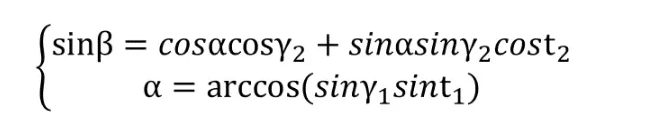
The specific process can be obtained by simply drawing a diagram and performing calculations. Therefore, I won’t go into detail here.
Given the constant angular velocities of the Earth’s rotation and revolution at any moment, the daily mean solar insolation coefficient at latitude A (A = 180*(π/2-γ2)/π, positive for northern and negative for southern latitudes) for a specific phase of revolution (season) t1, is the integral over the rotational phase (time of day) t2 in [0,2π] of the solar insolation coefficient at a point on this latitude, divided by 2π. The annual mean of the daily mean solar insolation coefficient is then the integral of the daily mean solar insolation coefficient over one year of the Earth’s revolution phase t1 in [0,2π], divided by 2π. Expressed in a formula, it would be:
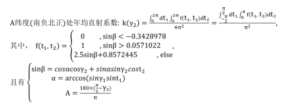
This involves a double integral of a piecewise function, and depending on the values of and , it requires different cases to be considered. If we were to express it as a single formula, then in one of these cases, the expression would be as follows:
When γ1, γ2 satisfy: for any t1, the minimum value of f(t1, t2) is 0 and the maximum value of f(t1, t2) is 1, the original expression can be written as k(γ2) =

The final annual average solar insolation coefficients for different latitudes under varying obliquity angles can only be computed either by a proficient mathematician or by a computer simulation. I am not the former, so I will have to write a program to simulate the integration results.
Here are the results for different latitudes under various obliquity angles:
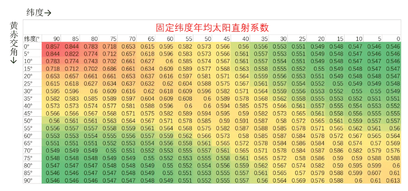
In the figure, the top row of numbers represents the latitudes where solar panels are located, with intervals of 5° from the poles to the equator. The leftmost column represents the planet’s obliquity.
It can be observed that as the obliquity increases, the annual average solar insolation at the poles decreases, while it increases at the equator. The area near the latitude of “100°-obliquity” is where the annual average solar insolation on Earth is maximized.
Therefore, when someone asks, “Where can solar panels be placed to maximize the total electricity generation over the year,” the answer is neither at the equator nor at the poles but at the latitude corresponding to 100°-obliquity.
Additionally, the figure reveals other insights. For instance, on planets with nearly zero obliquity, the solar energy generation at the poles exceeds that at the equator by over 50%. Moreover, for a planet with a horizontally oriented rotation axis, the maximum annual solar insolation is only around 60%, making it unsuitable for solar panel deployment.
Annual Average Insolation of the “Solar Cap” at Specific Latitudes
For blueprints tailored to one’s own game save, it is advisable, as mentioned in Section Two, to place them near the latitude of 100°-obliquity. However, for general-purpose usage, many players may prefer to sacrifice some efficiency optimization and use a more universally applicable set of polar solar panel blueprints. Hence, determining the electricity generation of polar solar blueprints at specific latitudes becomes necessary. The solar insolation from the poles to a particular latitude is the integral of the daily insolation at each latitude multiplied by the area of that latitude band. However, due to the high computational complexity involved, a rough estimation method is employed here. The method calculates the average of the upper and lower bounds of the latitude region multiplied by the area and then sums up these values for each 5° segment of Earth, dividing the total by the Earth’s surface area. The results are presented in the table below.
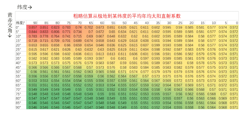
This approach reveals that for polar solar energy, the smaller the obliquity, the larger the annual average solar insolation. When covering from the poles to the equator with solar panels, the computed result using this method falls within the range of 0.571 to 0.572, with an error margin of less than 0.1% compared to the theoretical value mentioned in Section One. To validate the accuracy of this rough estimation method, I directly substituted the upper and lower bounds of the annual average solar insolation at high latitudes or low dimensions for the regional solar insolation. The absolute error between the upper and lower bounds obtained through rough estimation does not exceed 0.01. The specific table results have been provided in the “Dyson Sphere Project Numerical Calculation Statistics.”
Minimum Annual Average Insolation of the “Solar Cap” at Specific Latitudes
Considering practical scenarios where solar energy is the primary power source without using hubs (the reasons for not using hubs are complex and may require a separate discussion in another article), the actual usable electricity generated from solar energy over the year differs from the total annual electricity generation. Only when excess factories are placed to keep the production lines in a constant state of power shortage do we effectively utilize all the electricity generated by solar panels. However, deploying excess factories effectively reduces the efficiency of factory buildings, essentially trading off building efficiency for solar panel efficiency. Moreover, letting solar panel output determine production capacity results in imbalanced production capacity. Therefore, it is more practical to focus on the minimum daily electricity generation of the solar sphere until viable solutions for utilizing surplus electricity are suggested.
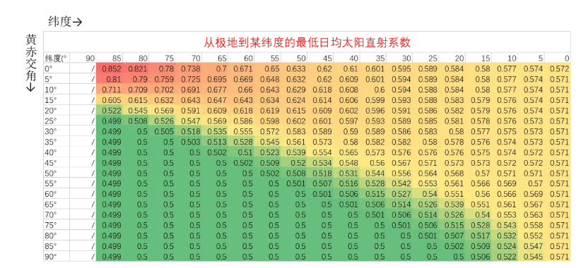
When a planet has a certain obliquity, for a solar cap covering from the poles symmetrically to a certain latitude on Earth, the highest electricity generation occurs during the equinoxes, while the lowest occurs during the solstices. (After careful consideration, I have decided not to provide the proof here. Constructing the proof involves many ad hoc concepts, making it difficult to describe and understand, and it is unlikely to be read extensively. It is recommended that readers think through the proof themselves, and if there are any questions, they can ask directly in the comments. Here’s a hint for the proof process:
- Consider the symmetry between the northern and southern hemispheres at the same latitude during the process of revolution and rotation.
- Consider the sum of the solar insolation coefficients of regions where the solar altitude angles are mutually opposite (decreasing from the equator towards both sides of the equinox line). Due to symmetry, the sum of 1 can be ignored, and the part greater than 1 is the actual contributor to the annual average solar insolation exceeding 50%. Let’s temporarily call it the “boundary gain region.” Consider how the intersection of the polar solar energy and this boundary gain region changes as the latitude of the zenith point increases.) Thus, by fixing t1 in the previous formula for “annual average daily solar insolation at a certain latitude” to π/2, we obtain the “minimum daily solar insolation at a certain latitude.” Then, integrating over latitude yields the results shown in the table below, which can be interpreted as the minimum daily solar insolation at different latitudes on planets with different scales of polar solar energy and varying obliquities or as the variation in daily solar insolation over a year on a planet with horizontally oriented rotation axis.
Sungold Solar conducted tests to further analyze solar panel orientation’s impact on energy production, yielding the following insights:
- At the same location, changes in azimuth orientation, whether facing east or west, have identical effects on power generation; meaning, installations facing east or west yield similar energy outputs.
- The reduction in power generation follows a parabolic trend; as the azimuth angle increases from 0°, the rate of energy loss accelerates.
- The variation in power generation is significantly affected by geographic location. In high-latitude areas, panels oriented east or west can experience energy losses exceeding 20%, whereas in low-latitude regions, losses are limited to around 4%.
- The loss in power generation due to changes in azimuth orientation is largely independent of longitude but is significantly correlated with latitude. Higher latitudes result in greater losses, while lower latitudes see reduced losses.
Customers can increase solar efficiency by finding the perfect solar panel angles. Stay up to date with Sungold Solar for more tips and knowledge on maximizing solar panel performance.